Oracle Manufacturing uses dynamic (quantity dependent) lead times to plan material and resource requirements, and to determine material requirement dates for available to promise (ATP) calculations. When computing requirement dates, both the fixed and variable components of an item's manufacturing lead time are used. When setting time fences for planning and available to promise calculations, an item's cumulative lead times are used.
For manufactured items, you can automatically compute manufacturing and cumulative lead times for a specific item or a range of items. You can also maintain this information manually. You must manually assign all lead time information for purchased items.
Note: You can calculate manufacturing and cumulative lead times for manufacturing or engineering items.
Updating the values assigned to your lead times may impact functions that use dynamic lead time offsetting- such as material and resource requirements planning. Updating cumulative lead times can also impact material plans and available to promise calculations if these lead times are used to set time fences.
For all scheduled time elements, which are less than the standard workday, the system will compute the lead time day by dividing the lead time element by 24. The standard workday is defined in the workday calendar. Oracle Manufacturing stores the following lead time information for each item:
Fixed Lead Time: The portion of manufacturing lead time that is independent of order quantity. You can enter this factor manually for an item, or compute it automatically for manufactured items.
Variable Lead Time: The portion of manufacturing lead time that is dependent on order quantity. You can enter this factor manually for an item, or compute it automatically for manufactured items.
Preprocessing Lead Time: A component of total lead time that represents the time required to release a purchase order or create a job from the time you learn of the requirement. You can manually enter preprocessing lead time for both manufactured and purchased items.
Post Processing Lead Time: A component of total lead time that represents the time to make a purchased item available in inventory from the time you receive it. Manually enter postprocessing lead time for each purchased item. Postprocessing lead time for manufactured items is not recognized.
Processing Lead Time: The time required to procure or manufacture an item. You can compute processing lead time for a manufactured item, or manually assign a value. Processing lead time is computed as the time as total integer days required to manufacture 1 lead time lot size of an item. You must manually assign a processing lead time for purchased items. Processing lead time does not include preprocessing and postprocessing lead times.
Lead Time Lot Size: The quantity you use to calculate manufacturing lead times. You can specify an item's lead time lot size to be different from the standard lot size.
Dynamic Lead Time Offsetting: A scheduling method that quickly estimates the start date of an order, operation, or resource. Dynamic lead time offsetting schedules using the organization workday calendar.
Total Lead Time: The fixed lead time plus the variable lead time multiplied by the order quantity. The planning process uses the total lead time for an item in its scheduling logic to calculate order start dates from order due dates.
Cumulative Manufacturing Lead Time: The total time required to make an item if you had all raw materials in stock but had to make all subassemblies level by level. Oracle Bills of Material automatically calculates this value, or you can manually assign a value.
Cumulative Total Lead Time: The total time required to make an item if no inventory existed and you had to order all the raw materials and make all subassemblies level by level. Bills of Material automatically calculates this value, or you can manually assign a value.
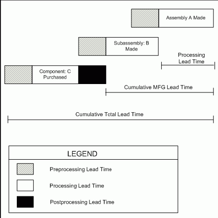
As described in the text above, the following diagram illustrates the relationship between preprocessing, processing, and postprocessing lead times for manufactured items (assembly A and subassembly B) and purchased items (component C). This diagram also describes the cumulative manufacturing lead time and cumulative total lead time for a manufactured item (assembly A).
Bills of Material computes manufacturing lead times from item, routing and resource availability information. Item and routing information is updated as part of the computation.
Processing lead time is computed as the time required to complete 1 lead time lot size of an item (the time required to complete the second scheduled job). Bills of Material determines an item's lead time lot size from two item master fields: standard lot size and lead time lot size.
For items that you plan and cost by the same lot size, you can specify a value only for the standard lot size. Bills of Material then computes manufacturing lead time using the standard lot size quantity.
Note: If an item's routing references another item's routing as a common, set both items' lead time lot size to the same value. If you do not specify a lead time lot size, ensure that both items' standard lot sizes are equal.
For items that you plan with one lot size and cost with a different lot size, you can enter a lead time lot size. Bills of Material then calculates manufacturing lead time using this value (rather than the standard lot size). If an item does not have a value for the standard or lead time lot size, Bills of Material uses a quantity of one to compute manufacturing lead times.
Note: If you enter a lead time lot size for an item, consider the item's planning lot size to accurately offset lead times. For planned items with a fixed order quantity, set the lead time lot size to the fixed order quantity. If a planned item has varying lot sizes, assign a lead time lot size that represents the typical lot size.
Oracle Manufacturing uses routing, operation, and resource information to compute fixed, variable, and processing lead times for manufactured items. Lead times are not calculated for purchased items even if they have a routing.
When computing manufacturing lead times, primary routings are automatically updated with lead time and offset percents. As with the item lead time attributes, you can also manually assign these values.
Oracle Manufacturing stores the lead time percent for each routing operation as the percent of manufacturing (processing) lead time required for previous operations, calculated from the start of a job to the start of an operation.
For example, if an item's manufacturing lead time is two days and the primary routing has two operations with the same duration (1 day), the first operation's lead time percent is zero and the second operation's lead time percent is 50%.
Oracle Manufacturing stores the offset percent for each resource on a routing operation as the percent of manufacturing (processing) lead time required for previous operations, calculated from the start of the job to the start time of a resource at an operation.
For example, both operations in the previous example for lead time percent require one day (eight hours) to perform. If you have two different resources assigned to the second operation, and each resource requires four hours to complete their task, the offset percent is 50% for the first resource and 75% for the second resource.
You can automatically compute processing, fixed, and variable lead times for manufactured items, whether they are produced using discrete jobs or repetitive schedules.
A value of zero is assigned to the fixed, variable, and processing lead times of a manufactured item that does not have a routing and is not assigned to a production line.
Discrete Jobs Lead Times
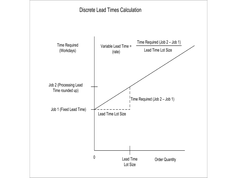
Bills of Material computes manufacturing lead time by forward scheduling two jobs: the first job is scheduled for a quantity of zero and the second job is scheduled for a quantity equal to the item's lead time lot size. The first job determines the fixed lead time and the second job determines the variable and processing lead times.
The second job's duration rounded up to an integer value represents the Processing Lead Time (in days). The difference between the duration of the second job and the duration of the first job divided by the Lead Time Lot Size represents the Variable Lead Time. Generally, the duration of the first job is 0 or very close to 0, hence, the Variable Lead Time variation based on Lead Time Lot Size changes may not be observable.
Variable Lead Time (rate) = (Job2 Duration - Job1 Duration)/Lead Time Lot Size.
Job1 Duration = the time required to complete a job for 0 quantity (and it represents the Fixed Lead Time).
Job2 Duration = the time required to complete a job for a quantity equal to the assembly item's Lead Time Lot Size (this value rounded up to an integer value represents the Processing Lead Time in days).
The following diagram illustrates discrete lead times calculation, as described in the text above:
Attention: Although Bills of Material uses detailed scheduling to compute lead times, all calendar days are considered workdays regardless of days off, workday exceptions, or shift exceptions.
Additional Information: Resource availability is calculated based on the average shift capacity. Shifts assigned to a resource typically specify work shift patterns. If the shift patterns change on different days, the sum of the total hours available across all shifts in a day is usually the same. If the total hours is different, Oracle uses the average total hours per work day.
Example
In the following example, Oracle Bills of Material assumes that the resource availability for Resource A is 8 hours ((10 + 10 + 4)/3 = 8).
| Operation | Resource | Shift | Shift Hours | Day |
|---|---|---|---|---|
| Operation 10 | Resource A | Shift 1 | 00:00 - 05:00 | Monday |
| Operation 10 | Resource A | Shift 2 | 08:00 - 13:00 | Monday |
| Operation 10 | Resource A | Shift 3 | 08:00 - 18:00 | Tuesday |
| Operation 10 | Resource A | Shift 4 | 10:00 - 14:00 | Wednesday |
| Operation 10 | Resource B | Shift 5 | 06:00 - 18:00 | Wednesday |
The resource availability for Resource A is calculated as 8 hours ((10 + 10 + 4)/3 = 8). Notice that the shift hours defined for the same workday (Monday) were added together and the resource availability is an average. In this case, if the resource usage rate is 10 hours for Resource A and 12 hours for Resource B, then the variable leadtime is calculated as 10/8 + 12/12 = 2.25 days. This number is reasonable because if an actual job to produce this assembly was scheduled over a Wednesday, it would take slightly more than 2 days to produce the assembly. On Wednesdays, there is only 6 hours of availability as opposed to the normal 10 hour shifts during the other workdays.
Additional Information: You cannot schedule a resource unless all prior quantities scheduled have been completed.
Sequential operations and resources assume that all quantities are scheduled in their entirety through a resource before the next quantity is scheduled to begin. For example, the time scheduled for two resources cannot overlap on a given day. However, when you schedule the job, the leadtime is slightly longer than you expected:
Operation 10
| Resource | Usage Rate (Hours) | Shift Assigned |
|---|---|---|
| 1 | 3 | 00:00 - 03:00 |
| 2 | 3 | 05:00 - 08:00 |
There is no fixed leadtime and the leadtime lot size is 2. The variable leadtime is 2 days because you need to complete the entire quantity of 2 (which takes 2 days) before you can start the second resource.
Bills of Material uses the following formulas to compute fixed and variable lead times:
Schedule a job for zero quantity beginning on the system date and compute fixed lead time as follows:
completion date (of one item) - system date
Schedule a job for the lead time lot size beginning on the system date and compute variable lead time (rate) as follows:
[(completion date (of all items) - system date) - fixed lead time] / lead time lot size
Repetitive Schedule Lead Times
A lead time lot size of 1 is always used to compute lead times for items produced on routing-based schedules.
The following terms apply to repetitive schedules:
Day: A day is equal to the number of hours the production line is active. If the line is active from 8:00 to 16:00, the day is 8 hours long.
Production Rate (Line Speed): The number of assemblies built per line, per hour.
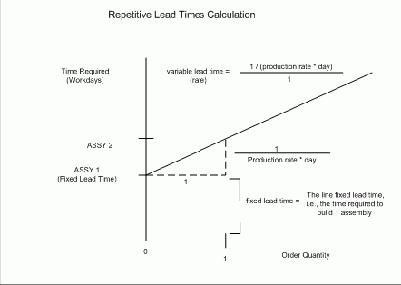
Line Fixed Lead Time: The fixed lead time of the production line, that is, the amount of time for one assembly to travel down a production line.
Production Interval: The time between two assemblies on a production line. If the production rate (line speed) is 10 assemblies per hour, then the production interval is .1 hours or once every .0125 days, or 1/(10*8), for a line that runs 8 hours per day. 1 / (production rate * day)
The Calculate Manufacturing Lead Times program calls the scheduler twice, first using a quantity of 1, then using a quantity of 0. For each case, the scheduling lead time (expressed in days) is returned. This is the total time taken to build the assemblies. The program then converts the two values into the fixed lead time and the variable lead time item attributes, respectively.
The following table illustrates how scheduling lead times are calculated:
| Assembly's Routing | Scheduling Basis | Quantity | Scheduling Lead Time |
|---|---|---|---|
| No routing | routing | 0 | 0 |
| No routing | routing | 1 | production interval |
| No routing | fixed | 0 | line fixed lead time |
| No routing | fixed | 1 | line fixed lead time + production interval |
| Assembly with item-based resources only | routing | 0 | fixed lead time - production interval |
| - | routing | 1 | (fixed lead time - production interval) + production interval |
| - | fixed | 0 | line fixed lead time |
| - | fixed | 1 | line fixed lead time + production interval |
| Assembly with item- and lot- based resources | routing | 0 | fixed lead time - production interval |
| - | routing | 1 | (fixed lead time - production interval) + production interval |
| - | fixed | 0 | line fixed lead time |
| - | fixed | 1 | line fixed lead time + production interval |
For fixed lead time lines, the fixed and variable lead times are not based on whether a routing exists. The fixed lead time is always the line fixed lead time, the amount of time for one assembly to travel down a production line. The variable lead time is always the production interval:
variable lead time (repetitive schedule) = 1 / (production rate * day)
For a routing-based line, the fixed lead time is the time required to build one assembly; the fixed lead time includes the time for both item and lot-based resources.
The following diagram illustrates repetitive lead times calculation, as described in the text above:
Bills of Material also computes the processing lead time as the time required to complete the second scheduled job (where the job starts on the system date):
completion date (of one item) - system date
Processing lead time is presented in whole days rounded to the next day.
ExampleFor example, if for item A, you had the following data:
Lead time lot size = 10 units
System date = 01-JAN
End date for work in process job for 1 unit = 10-JAN
End date for work in process job for 10 units = 13-JAN
Then:
| fixed lead time = | completion date (of one item) - system date |
| fixed lead time = | = 10-JAN - 01-JAN |
| fixed lead time = | = 10 days |
| Variable lead time = | [(completion date - system date) (rate) - fixed lead time] / lead time lot size |
| Variable lead time = | [(13-JAN - 01-JAN) - 10] / 10 |
| Variable lead time = | [13 - 10] / 10 |
| Variable lead time = | 0.3 days/unit |
| Processing lead time = | completion date - system date |
| Processing lead time = | 13-JAN - 01-JAN |
| Processing lead time = | 13 days |
The corresponding operation lead time percent for operations in the primary routing is updated automatically.
For example, if the routing operations for item A had the following start dates (on a job for 10 assemblies), Bills of Material would compute and update the following operation lead time percentages, as shown in the table below:
Operation Lead Time Percent
| Op Seq | Start Date and Time | End Date and Time | Time Required | Previous Op Time Required | Lead Time Percent |
|---|---|---|---|---|---|
| 10 | 01-JAN - 00:00 | 02-JAN - 24:00 | 2 | 0 | 0/10 = 0% |
| 20 | 03-JAN - 00:00 | 04-JAN - 24:00 | 2 | 2 | 2/10 = 20% |
| 30 | 05-JAN - 00:00 | 09-JAN - 24:00 | 4 | 4 | 4/10 = 40% |
| 40 | 09-JAN - 00:00 | 10-JAN - 24:00 | 2 | 8 | 8/10= 80% |
Bills of Material also computes, for each operation resource in an item's primary routing, the percent of total lead time required for previous resource operations in that routing.
For example, if your resource start and end times were as follows, Bills of Material would compute these resource offset percents, as shown in the table below:
Resource Offset Percent
| Op Seq | Res. Seq | Start Date and Time | End Date and Time | Time Required | Previous Res Time Required | Offset Percent |
|---|---|---|---|---|---|---|
| 10 | 1 2 | 01-JAN - 00:00 02-JAN - 00:00 | 01-JAN - 24:00 02-JAN - 24:00 | 1 1 | 0 1 | 0/10 = 0% 1/10 = 10% |
| 20 | 1 | 03-JAN - 00:00 | 04-JAN - 24:00 | 2 | 2 | 2/10 = 20% |
| 30 | 1 2 | 05-JAN - 00:00 07-JAN - 00:00 | 06-JAN - 24:00 08-JAN - 24:00 | 2 2 | 4 6 | 4/10 = 40% 6/10 = 60% |
| 40 | 1 | 09-JAN - 00:00 | 10-JAN - 24:00 | 2 | 8 | 8/10= 80% |
Bills of Material computes cumulative manufacturing lead time and cumulative lead time by stepping through indented bill structures. Item information is updated as part of the both cumulative calculations.
Bills of Material sets an item's cumulative manufacturing lead time equal to its own manufacturing lead time plus the maximum value of the cumulative manufacturing lead time for any component, adjusted for operation offset. The operation offset is the lead time percent for the operation where the component is used times the item's manufacturing lead time (based on one lead time lot size).
Purchasing items have no cumulative manufacturing lead time.
Bills of Material uses the following formula to compute cumulative manufacturing lead time:
manufacturing lead time for item + Maximum [(cumulative manufacturing lead time - offset days) for any component]
Bills of Material sets an item's cumulative total lead time to its own total lead time plus the maximum value of cumulative total lead time less operation offset for any component. Operation offset for a component is the lead time percent for the operation where the component is used times the item's manufacturing lead time (based on one lead time lot size).
Bills of Material calculates cumulative total lead time using the following equation:
total lead time for item + Maximum [(cumulative total lead time - offset days) for any component]
For example, suppose Item A is made up of B, C, and D. B, C, and D are used at operations 20, 30, and 40 respectively and the manufacturing (processing) lead time for A (for the lead time lot size) equals 10. The following table illustrates the component, offset days, and lead time percent for each component:
Cumulative Manufacturing Lead Time
| Component | Cum. Mfg. Lead Time. | Op Seq. | Lead Time Percent | Offset Days | Cum Mfg. Lead Time - Offset Days |
|---|---|---|---|---|---|
| B | 15 | 20 | 20 | 2 | 13 |
| C | 20 | 30 | 40 | 4 | 16 |
| D | 22 | 40 | 80 | 8 | 14 |
Bills of Material calculates cumulative manufacturing lead time as follows:
manufacturing lead time for A + Maximum [(cumulative manufacturing lead time - offset days) for component B, C, or D]
Cumulative manufacturing lead time = 10 + 16 = 26 days
The following table illustrates the cumulative total lead times assigned to components B, C, and D:
Cumulative Total Lead Time
| Component | Cum. Total Lead Time. | Op Seq. | Lead Time Percent | Offset Days | Cum Total Lead Time - Offset Days |
|---|---|---|---|---|---|
| B | 19 | 20 | 20 | 2 | 17 |
| C | 20 | 30 | 40 | 4 | 16 |
| D | 23 | 40 | 80 | 8 | 15 |
Bills of Material calculates cumulative total lead time for A as follows:
total lead time for A + Maximum [(cumulative total lead time - offset days) for component B, C, or D]
Cumulative total lead time = 10 + 17 = 27 days
Other Sources
Overview of Material Requirements Planning, Oracle MRP User's Guide